Plot First Differences from MCMC output

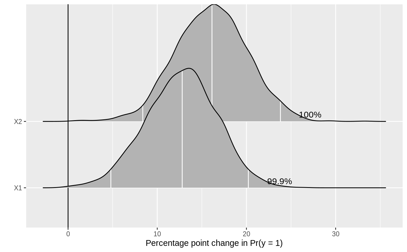
R function to plot first differences generated from MCMC output. For more on this method, see the documentation for mcmcFD(), Long (1997, Sage Publications), and King, Tomz, and Wittenberg (2000, American Journal of Political Science 44(2): 347-361). For a description of this type of plot, see Figure 1 in Karreth (2018, International Interactions 44(3): 463-90).

mcmcFDplot(fdfull, ROPE = NULL)

Arguments

fdfull	Output generated from mcmcFD(..., full_sims = TRUE).
ROPE	defaults to NULL. If not NULL, a numeric vector of length two, defining the Region of Practical Equivalence around 0. See Kruschke (2013, Journal of Experimental Psychology 143(2): 573-603) for more on the ROPE.

Value

a density plot of the differences in probabilities. The plot is made with ggplot2 and can be passed on as an object to customize. Annotated numbers show the percent of posterior draws with the same sign as the median estimate (if ROPE = NULL) or on the same side of the ROPE as the median estimate (if ROPE is specified).

Details

An R function to plot first differences after a Bayesian logit or probit model.

References

• Karreth, Johannes. 2018. “The Economic Leverage of International Organizations in Interstate Disputes.” International Interactions 44 (3): 463-90. https://doi.org/10.1080/03050629.2018.1389728.

• King, Gary, Michael Tomz, and Jason Wittenberg. 2000. “Making the Most of Statistical Analyses: Improving Interpretation and Presentation.” American Journal of Political Science 44 (2): 347–61. http://www.jstor.org/stable/2669316.

• Kruschke, John K. 2013. “Bayesian Estimation Supersedes the T-Test.” Journal of Experimental Psychology: General 142 (2): 573–603. https://doi.org/10.1037/a0029146.

• Long, J. Scott. 1997. Regression Models for Categorical and Limited Dependent Variables. Thousand Oaks: Sage Publications.

Examples

.old_wd <- setwd(tempdir())
# \donttest{
## simulating data
set.seed(123456)
b0 <- 0.2 # true value for the intercept
b1 <- 0.5 # true value for first beta
b2 <- 0.7 # true value for second beta
n <- 500 # sample size
X1 <- runif(n, -1, 1)
X2 <- runif(n, -1, 1)
Z <- b0 + b1 * X1 + b2 * X2
pr <- 1 / (1 + exp(-Z)) # inv logit function
Y <- rbinom(n, 1, pr)
data <- data.frame(cbind(X1, X2, Y))

## formatting the data for jags
datjags <- as.list(data)
datjags$N <- length(datjags$Y)

## creating jags model
model <- function()  {

  for(i in 1:N){
    Y[i] ~ dbern(p[i])  ## Bernoulli distribution of y_i
    logit(p[i]) <- mu[i]    ## Logit link function
    mu[i] <- b[1] +
      b[2] * X1[i] +
      b[3] * X2[i]
  }

  for(j in 1:3){
    b[j] ~ dnorm(0, 0.001) ## Use a coefficient vector for simplicity
  }

}

params <- c("b")
inits1 <- list("b" = rep(0, 3))
inits2 <- list("b" = rep(0, 3))
inits <- list(inits1, inits2)

## fitting the model with R2jags
set.seed(123)
fit <- R2jags::jags(data = datjags, inits = inits,
                    parameters.to.save = params, n.chains = 2, n.iter = 2000,
                    n.burnin = 1000, model.file = model)
#> Compiling model graph
#>    Resolving undeclared variables
#>    Allocating nodes
#> Graph information:
#>    Observed stochastic nodes: 500
#>    Unobserved stochastic nodes: 3
#>    Total graph size: 3506
#> 
#> Initializing model
#> 

## preparing data for mcmcFD()
xmat <- model.matrix(Y ~ X1 + X2, data = data)
mcmc <- coda::as.mcmc(fit)
mcmc_mat <- as.matrix(mcmc)[, 1:ncol(xmat)]

## plotting with mcmcFDplot()
full <- mcmcFD(modelmatrix = xmat,
               mcmcout = mcmc_mat,
               fullsims = TRUE)
mcmcFDplot(full)
#> Picking joint bandwidth of 0.00785

# }

setwd(.old_wd)